Background Models

ShirleyBG

class lmfitxps.models.ShirleyBG(*args, **kwargs)

Model of the Shirley background for X-ray photoelectron spectroscopy (XPS) spectra. This implementation calculates the Shirley background by integrating the step characteristic of the spectrum. For further details, please refer to Shirley [6] or Jansson et al. [7].

The Shirley background is calculated using the following integral:

(4)\[B_S(E)=k\cdot \int_{E}^{E_{\text{right}}}\left[I(E')-I_{\text{right}}\right] \, dE'\]

The Shirley background is typically calculated iteratively using the following formula:

(5)\[B_{S, n}(E) = k_n \cdot \int_{E}^{E_{\text{right}}} [I(E') - I_{\text{right}} - B_{S, n-1}(E')] \, dE'\]

The iterative process continues until the difference \(B_{S, n}(E) - B_{S, n-1}(E)\) becomes smaller than a specified tolerance value \(tol\). This approach is implemented in the function referenced as shirley_calculate().

However, calculating the Shirley background before fitting and calculating it with high precision in each fitting step are not practically meaningful. Instead, the Shirley background is computed according to the equation (4) within each iteration of the model optimization. This ensures that the Shirley background is adaptively determined during the fitting process, preserving the iterative concept of its calculation.

Table 4 Model-specific available parameters

Parameters	Type	Description
x	array	1D-array containing the x-values (energies) of the spectrum.
y	array	1D-array containing the y-values (intensities) of the spectrum.
k	float	Shirley parameter \(k\), determines step-height of the Shirley background.
const	float	Constant value added to the step-like Shirley background, often set to \(I_{\text{right}}\).

Hint

The ShirleyBG class inherits from lmfit.model.Model and acts as a predefined model for calculating the Shirley background.Therefore, the lmfit.model.Model class parameters are inherited as well.

LMFIT: Common models documentation

Parameters:

• independent_vars (list of str, optional) – Arguments to the model function that are independent variables default is [‘x’]).

• prefix (str, optional) – String to prepend to parameter names, needed to add two Models that have parameter names in common.

• nan_policy ({'raise', 'propagate', 'omit'}, optional) – How to handle NaN and missing values in data. See Notes below.

• **kwargs (optional) – Keyword arguments to pass to Model.

Notes

1. nan_policy sets what to do when a NaN or missing value is seen in the data. Should be one of:

• ‘raise’ : raise a ValueError (default)

• ‘propagate’ : do nothing

• ‘omit’ : drop missing data

Note

The class functions are inherited from the lmfit Model class. For details, please refer to their documentation at lmfit Model Class Methods.

TougaardBG

class lmfitxps.models.TougaardBG(*args, **kwargs)

The TougaardBG model is based on the four-parameter loss function (4-PIESCS) as suggested by R.Hesse [1].

In addition to R.Hesse’s approach, this model introduces the extend parameter, which enhances the agreement between the data and the Tougaard background by extending the data on the high-kinetic energy side (low binding energy side) using the mean value of the rightmost ten intensity values (with regard to kinetic energy scale, binding energy scale vice versa).

The extend parameter represents the length of the data extension on the high-kinetic-energy side in eV and defaults to 0.

This approach was found to lead to great convergence empirically with the extend value being in the range of 25eV to 75eV; however, the length of the data extension remains arbitrary and depends on the dataset.

For further details, please read more in The ‘extend’ parameter in TougaardBG.

The Tougaard background is calculated using:

\[B_T(E) = \int_{E}^{\infty} \frac{B \cdot T}{{(C + C_d \cdot T^2)^2} + D \cdot T^2} \cdot y(E') \, dE'\]

where:

• \(B_T(E)\) represents the Tougaard background at energy \(E\),

• \(y(E')\) is the measured intensity at \(E'\),

• \(T\) is the energy difference \(E' - E\).

• \(B\) parameter of the 4-PIESCS loss function as introduced by R.Hesse [1]. Acts as the scaling factor for the Tougaard background model.

• \(C\) , \(C_d\) and \(D\) are parameter of the 4-PIESCS loss function as introduced by R.Hesse [1].

To generate the 2-PIESCS loss function, set \(C_d\) to 1 and \(D\) to 0. Set \(C_d=1\) and \(D !=\) \(0\) to get the 3-PIESCS loss function.

For further details on the 2-PIESCS loss function, please refer to S.Tougaard [2], and for the 3-PIESCS loss function, see S. Tougaard [3].

Table 5 Model-specific available parameters

Parameters	Type	Description
x	array	1D-array containing the x-values (energies) of the spectrum.
y	array	1D-array containing the y-values (intensities) of the spectrum.
B	float	B parameter of the 4-PIESCS loss function [1].
C	float	C parameter of the 4-PIESCS loss function [1].
C_d	float	C’ parameter of the 4-PIESCS loss function [1].
D	float	D parameter of the 4-PIESCS loss function [1].
extend	float	Determines, how far the spectrum is extended on the right (in eV).

Hint

The TougaardBG class inherits from lmfit.model.Model and extends it with specific behavior and functionality related to the Tougaard 4-parameter loss function. Therefore, the lmfit.model.Model class parameters are inherited as well.

LMFIT: Common models documentation

Parameters:

• independent_vars (list of str, optional) – Arguments to the model function that are independent variables default is [‘x’]).

• prefix (str, optional) – String to prepend to parameter names, needed to add two Models that have parameter names in common.

• nan_policy ({'raise', 'propagate', 'omit'}, optional) – How to handle NaN and missing values in data. See Notes below.

• **kwargs (optional) – Keyword arguments to pass to Model.

Notes

1. nan_policy sets what to do when a NaN or missing value is seen in the data. Should be one of:

• ‘raise’ : raise a ValueError (default)

• ‘propagate’ : do nothing

• ‘omit’ : drop missing data

Note

The class functions are inherited from the lmfit Model class. For details, please refer to their documentation at lmfit Model Class Methods.

The ‘extend’ parameter in TougaardBG

The challenge in calculating an approximation to the Tougaard background involves the following:

The factor B is adjusted to give zero intensity in a region between 30 and 50 eV below the characteristic peak structure [4].

That’s due to:

[…] that the peaks extend to ∼30 eV on the low energy side of the characteristic peaks. The intensity in this energy range arises from the intrinsic (or shake-up) electrons. [4] [5]

However, in practice, measuring high-resolution spectra across such a broad energy range is typically unfeasible.

Due to the nature of the Tougaard background, one encounters the integral:

\[B_T(E) = \int_{E}^{\infty} \frac{B \cdot T}{{(C + C_d \cdot T^2)^2} + D \cdot T^2} \cdot y(E') \, dE'\]

It’s worth noting that the upper bound of the integral is set to \(\infty\). However, experimental data collection usually occurs within a finite energy range. Consequently, the need for suitable approximations to this integral arises.

A common approach is to limit the integral to the measured energy range. By doing so, the Tougaard integral approaches \(0\) for the rightmost energy values (depending on the choosen constant!), leading to an inaccurate approximation of the measured data. To address this issue, the background is modified using the following equation:

\[B(E) = B_T(E) + B_C\]

Here, \(B_C\) is a constant term. However, when dealing with substantial asymmetry in the observed peaks, we found empirically that this approach using an added constant does not lead to an accurate approximation of the background. To generate such a background, the TougaardBG -model could be used with extend set to \(0\) and an additional ConstantModel from lmfit.

import lmfit
import lmfitxps

tougaard_bg=lmfitxps.models.TougaardBG(prefix='tougaard_', independent_vars=['y', 'x'])
const_bg=lmfit.models.ConstantModel(prefix='const_')

bg_model=tougaard_bg+const_bg

params = lmfit.Parameters()
params.add('tougaard_extend', value=0)

# Set all other parameters

Using this background model, an Au4f spectrum was fitted. To model the dublett structure, a convolution of a gaussian with doniach profiles was used as implemented in ConvGaussianDoniachDublett.

All peaks parameters were fixed and not varied in the fit to make it possible to compare the effect of different values for the extend parameter.

As shown in the figure below, the combination of TougaardBG and ConstantModel already leads to a good agreement between fit and experimental data.

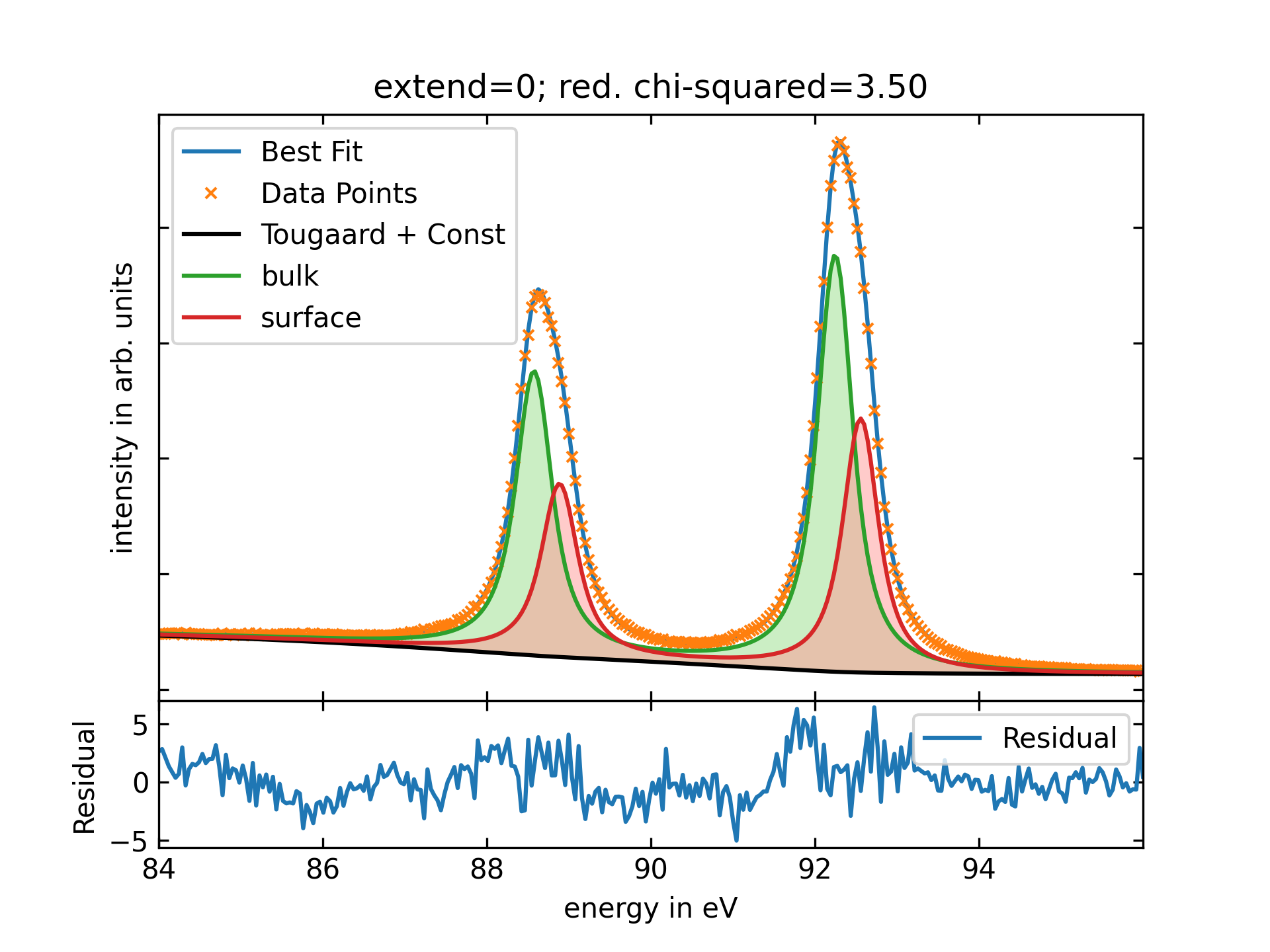
Due to the small asymmetry of the Au4f-signal only small improvement of the fit was achieved by using \(extend\) != \(0\). This is shown in the four figures below. The reduced chi-squared, which judges the agreement between model and experimental data, is only slightly decreased using \(28 \leq \text{extend} \leq 30\). In addition, the figure below confirms, that using the TougaardBG with \(extend!=0\) is valid for modeling the background too.

The following figure illustrates the difference between \(B_T(\text{extend}) - (B_T(\text{extend}=0) + B_C)\) and also displays the variation in residuals between models where \(\text{extend} \neq 0\) and the model with \(\text{extend} = 0\).

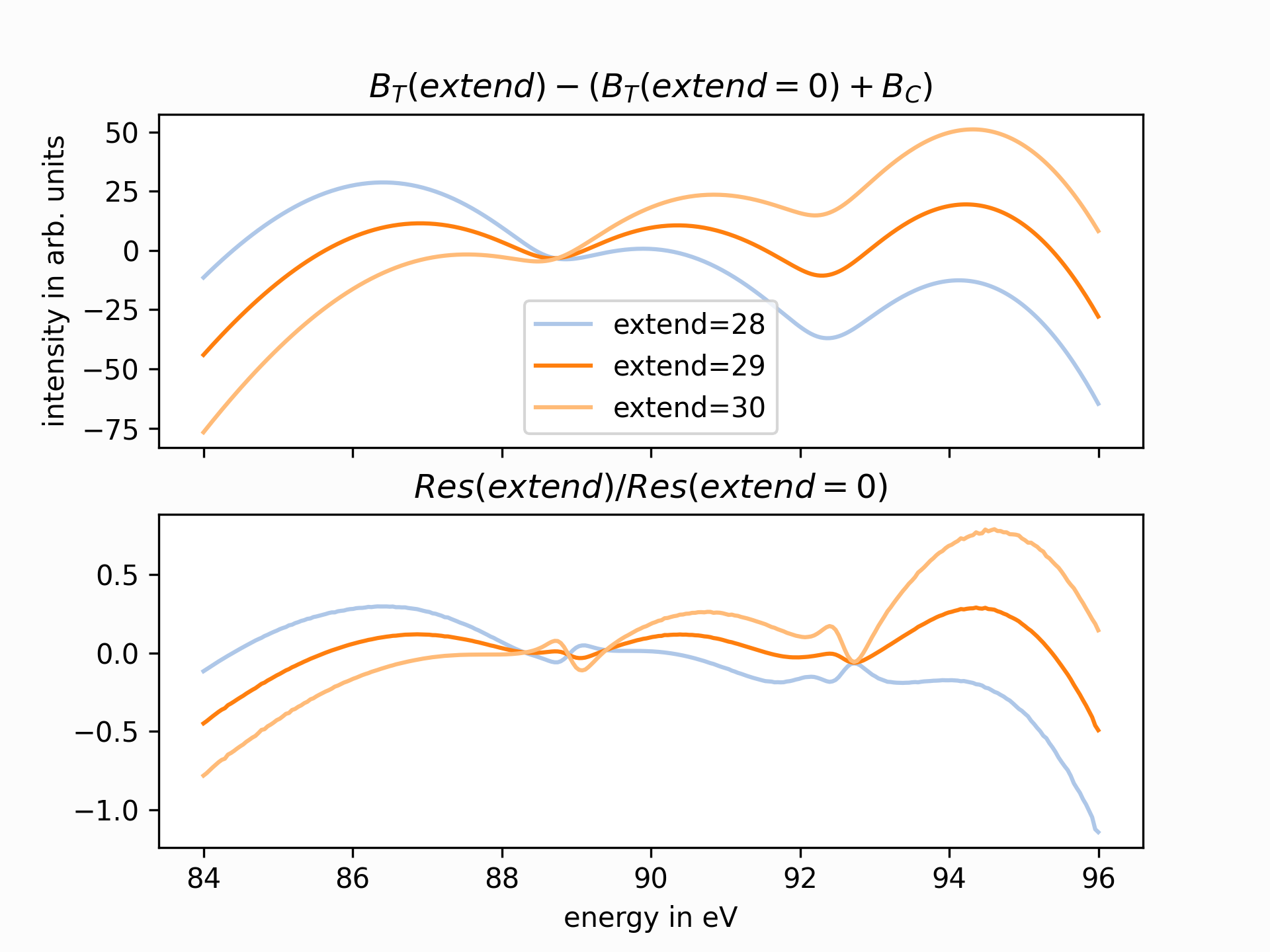
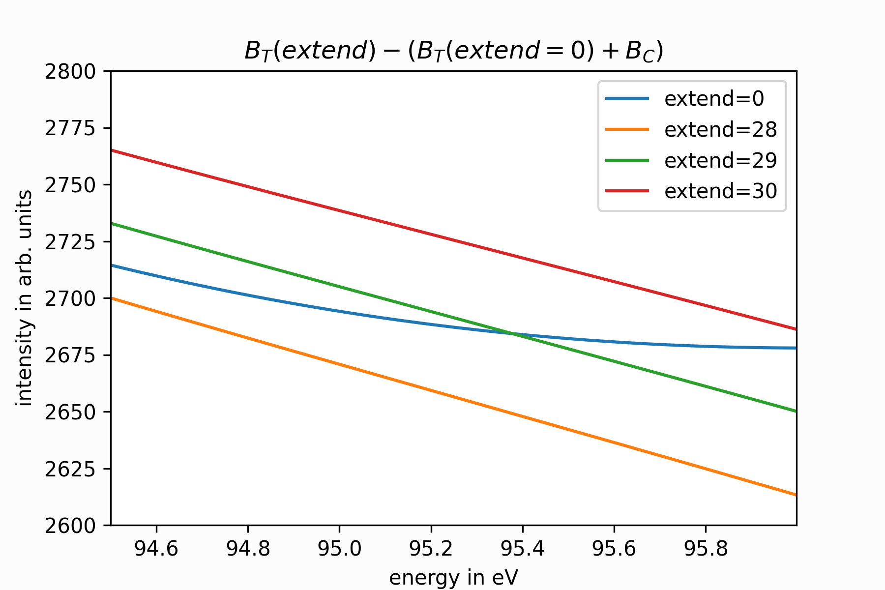
Clear patterns emerge among the backgrounds when :math:text{extend} neq 0, exhibiting a nearly linear behavior as they move away from the peak. In contrast, the model with :math:text{extend} = 0 displays a distinct parabolic shape, as illustrated in the figure below.

If the parabolic characteristic of the Tougaard background is too pronounced, the approximated Tougaard background with :math:text{extend} = 0 often intersects the data short below the fitted peak signal. This behavior does not fulfill the intended function of approaching the measured background around 30-50 eV on the low-energy side beneath the peak, which accounts for previously mentioned shake-up electrons.

Nevertheless, when compared to an average background value of approximately :math:I = 2700 counts, discrepancies among various models remain within a confined range of about 2%.

To see the source code for generating the extend-parameter plots, please expand:

import numpy as np
import matplotlib.pyplot as plt
import lmfit
import os
import sys
import os
sys.path.insert(0, os.path.abspath(os.path.join(os.path.dirname(__file__), '../src')))
from lmfitxps import models
import matplotlib as mpl
def guess_extend(x,y, B, C, C_d, D):
    y_end=np.mean(y[-10:])
    delta_x=(x[-1]-x[0])/len(x)
    tougaard_sum=0
    n=0
    lower=0
    lower_reached=False
    while B*tougaard_sum<y_end*0.9:
        n+=1
        tougaard_sum=0
        for j in range(n):
             tougaard_sum+= (j*delta_x) / ((C + C_d * (j*delta_x) ** 2) ** 2
                                              + D * (j*delta_x) ** 2) * y_end * delta_x
        if B*tougaard_sum>=y_end*0.5 and not lower_reached:
            lower=n
            lower_reached=True
    print('result, n={}, extend={}, lower={}'.format(n, n*delta_x, lower*delta_x))

exec_dir = os.path.abspath(os.path.join(os.path.dirname(__file__), '..'))
tougaard_model = models.TougaardBG(prefix='tougaard_', independent_vars=['y', 'x'])
d1 = models.ConvGaussianDoniachDublett(prefix='d1_')
d2 = models.ConvGaussianDoniachDublett(prefix='d2_')
const = lmfit.models.ConstantModel(prefix='const_')

data = np.genfromtxt(exec_dir + '/examples/clean_Au_4f.csv', delimiter=',', skip_header=1)
x = data[:, 0]
y = data[:, 1]
guess_extend(x,y,156.969,144.506,0.281,268.598)
output_dir = os.path.join(exec_dir, 'docs/src/', 'plots')
os.makedirs(output_dir, exist_ok=True)

combined_fig, (combined_ax1, combined_ax2) = plt.subplots(nrows=2,gridspec_kw={'height_ratios': [1, 1]}, sharex=True)
combined_fig.patch.set_facecolor('#FCFCFC')
residual_fig, residual_ax = plt.subplots(figsize=(6, 4))
residual_fig.patch.set_facecolor('#FCFCFC')
combined2_fig, combined2_ax = plt.subplots(figsize=(6, 4))
combined2_fig.patch.set_facecolor('#FCFCFC')
tg_bgs=[]
tg_res=[]
for j in [0]+[i for i in range(27,35,1)]:
    params = lmfit.Parameters()
    params.add('tougaard_B', value=148.969)
    params.add('tougaard_C', value=144.506, vary=False)
    params.add('tougaard_C_d', value=0.281, vary=False)
    params.add('tougaard_D', value=268.598, vary=False)
    params.add('tougaard_extend', value=j)
    params.add('d1_amplitude', value=71980, vary=False)
    params.add('d1_sigma', value=0.2126, vary=False)
    params.add('d1_gamma', value=0.01, vary=False)
    params.add('d1_gaussian_sigma', value=0.0892, vary=False)
    params.add('d1_center', value=92.2273, vary=False)
    params.add('d1_soc', value=3.67127, vary=False)
    params.add('d1_height_ratio', value=0.7, vary=False)
    params.add('d1_fct_coster_kronig', value=1.04, vary=False)
    params.add('d2_amplitude', value=43966, vary=False)
    params.add('d2_sigma', value=0.2, expr='d1_sigma')
    params.add('d2_gamma', value=0.0, expr='d1_gamma')
    params.add('d2_gaussian_sigma', value=0.14, expr='d1_gaussian_sigma')
    params.add('diff', value=0.31)
    params.add('d2_center', value=92.4, expr='d1_center+diff')
    params.add('d2_soc', value=3.67, expr="d1_soc")
    params.add('d2_height_ratio', value=0.7, expr='d1_height_ratio')
    params.add('d2_fct_coster_kronig', value=1, expr='d1_fct_coster_kronig')

    if j == 0:
        params.add('const_c', value=y[-1])
        fit_model = tougaard_model + d1+d2  + const
    else:
        fit_model = tougaard_model + d1+d2

    result = fit_model.fit(y, params, y=y, x=x, weights=1 /(np.sqrt(y)))
    comps = result.eval_components(x=x, y=y)
    fig, (ax1, ax2) = plt.subplots(nrows=2,gridspec_kw={'height_ratios': [4, 1]}, sharex=True)
    fig.patch.set_facecolor('#FCFCFC')
    # Data plot
    cmap = mpl.colormaps['tab20']
    ax1.plot(x, result.best_fit, label='Best Fit', color=cmap(0))
    ax1.plot(x, y, 'x', markersize=4, label='Data Points', color=cmap(2))
    if j == 0:
        ax1.plot(x, comps['const_'] + comps['tougaard_'], label='Tougaard + Const', color='black')
        ax1.plot(x, comps['d1_'] + comps['const_'] + comps['tougaard_'], color=cmap(4), label="bulk")
        ax1.plot(x, comps['d2_'] + comps['const_'] + comps['tougaard_'], color=cmap(6), label="surface")
        ax1.fill_between(x, comps['d1_'] + comps['const_'] + comps['tougaard_'], comps['const_'] +comps['tougaard_'], alpha=0.5,color=cmap(5))
        ax1.fill_between(x, comps['d2_'] + comps['const_'] + comps['tougaard_'], comps['const_'] +comps['tougaard_'], alpha=0.5,color=cmap(7))
        tg_bgs.append([comps['const_']+comps['tougaard_'], 0])
        tg_res.append([result.residual,0])
    else:
        if j>=28 and j<=30:
            tg_bgs.append([comps['tougaard_'], j])
            tg_res.append([result.residual, j])
        ax1.plot(x, comps['d1_'] + comps['tougaard_'], color=cmap(4), label="bulk")
        ax1.plot(x, comps['d2_'] + comps['tougaard_'], color=cmap(6), label="surface")
        ax1.fill_between(x, comps['d1_'] + comps['tougaard_'], comps['tougaard_'], alpha=0.5, color=cmap(5))
        ax1.fill_between(x, comps['d2_'] + comps['tougaard_'], comps['tougaard_'], alpha=0.5, color=cmap(7))
        ax1.plot(x, comps['tougaard_'], label='Tougaard')
    ax1.legend()
    ax1.set_xlabel('energy in eV')
    ax1.set_ylabel('intensity in arb. units')
    # Set ticks only inside
    ax1.tick_params(axis='x', which='both',top=True, direction='in')
    ax1.tick_params(axis='y', which='both', right=True,direction='in')
    ax2.tick_params(axis='x', which='both',top=True, direction='in')
    ax2.tick_params(axis='y', which='both', right=True, direction='in')
    #ax1.set_xticklabels([])
    ax1.set_yticklabels([])
    ax1.set_title(f'extend={j}; red. chi-squared='+"{:.2f}".format(result.redchi))
    plt.subplots_adjust(hspace=0)
    ax1.set_xlim(np.min(x), np.max(x))
    # Residual plot
    residual = result.residual
    ax2.plot(x, residual, label='Residual')
    ax2.legend()
    ax2.set_xlabel('energy in eV')
    ax2.set_ylabel('Residual')

    # Save individual plots
    plot_filename = os.path.join(output_dir, f'plot_{j}.png')
    plt.savefig(plot_filename, dpi=300)
    plt.close(fig)


    # Add residual to the combined residual plot
    residual_ax.plot(x, residual/np.sqrt(y), label=f'j={j}')

for i, item in enumerate(tg_bgs[1:], start=1):
    print(i, item[1])
    combined_ax1.plot(x, item[0] - tg_bgs[0][0], label='extend={}'.format(item[1]), color=cmap(i))

for i, item in enumerate(tg_res[1:], start=1):
    combined_ax2.plot(x, (item[0] - tg_res[0][0]), label='extend={}'.format(item[1]), color=cmap(i))
combined_ax1.legend()
combined_ax2.set_xlabel('energy in eV')
combined_ax1.set_ylabel('intensity in arb. units')
combined_ax1.set_title(r'$B_T(extend)-(B_T(extend=0)+B_C)$')
combined_ax2.set_title(r'$Res(extend)$/$Res(extend=0)$')
combined_plot_filename = os.path.join(output_dir, 'combined_plot.png')
combined_fig.savefig(combined_plot_filename, dpi=300)
plt.close(combined_fig)


for item in tg_bgs:
    combined2_ax.plot(x, item[0], label='extend={}'.format(item[1]))
combined2_ax.legend()
combined2_ax.set_ylim(2600,2800)
combined2_ax.set_xlim(94.5,np.max(x))
combined2_ax.set_xlabel('energy in eV')
combined2_ax.set_ylabel('intensity in arb. units')
combined2_ax.set_title(r'$B_T(extend)-(B_T(extend=0)+B_C)$')
combined2_plot_filename = os.path.join(output_dir, 'combined2_plot.png')
combined2_fig.savefig(combined2_plot_filename, dpi=300)
plt.close(combined2_fig)

residual_ax.legend()
residual_ax.set_xlabel('x')
residual_ax.set_ylabel('Residual')
residual_plot_filename = os.path.join(output_dir, 'combined_residual_plot.png')
residual_fig.savefig(residual_plot_filename, dpi=300)
plt.close(residual_fig)

# with binding energy
data = np.genfromtxt(exec_dir + '/examples/clean_Au_4f.csv', delimiter=',', skip_header=1)

x = 180-data[:, 0]
y = data[:, 1]
output_dir = os.path.join(exec_dir, 'docs/src/', 'plots')
os.makedirs(output_dir, exist_ok=True)




params = lmfit.Parameters()
params.add('tougaard_B', value= 197.643926)
params.add('tougaard_C', value=144.506, vary=False)
params.add('tougaard_C_d', value=0.281, vary=False)
params.add('tougaard_D', value=268.598, vary=False)
params.add('tougaard_extend', value=0)
params.add('d1_amplitude', value=71980)
params.add('d1_sigma', value=0.21)
params.add('d1_gamma', value=0.01)
params.add('d1_gaussian_sigma', value=0.0892)
params.add('d1_center', value=180-92.2273)
params.add('d1_soc', value=3.67127)
params.add('d1_height_ratio', value=0.7)
params.add('d1_fct_coster_kronig', value=1.04, vary=False)
params.add('d2_amplitude', value=43966)
params.add('d2_sigma', value=0.2, expr='d1_sigma')
params.add('d2_gamma', value=0.0, expr='d1_gamma')
params.add('d2_gaussian_sigma', value=0.14, expr='d1_gaussian_sigma')
params.add('diff', value=-0.31165)
params.add('d2_center', value=180-92.4, expr='d1_center+diff')
params.add('d2_soc', value=-3.67, expr="d1_soc")
params.add('d2_height_ratio', value=0.7, expr='d1_height_ratio')
params.add('d2_fct_coster_kronig', value=1, expr='d1_fct_coster_kronig')
params.add('const_c', value=2677.97771)
fit_model = tougaard_model + d1+d2  + const

result = fit_model.fit(y, params, y=y, x=x, weights=1 /(np.sqrt(y)))
comps = result.eval_components(x=x, y=y)
fig, (ax1, ax2) = plt.subplots(nrows=2,gridspec_kw={'height_ratios': [4, 1]}, sharex=True)
fig.patch.set_facecolor('#FCFCFC')
# Data plot
cmap = mpl.colormaps['tab20']
ax1.plot(x, result.init_fit, label='Init Fit', color=cmap(3))
ax1.plot(x, result.best_fit, label='Best Fit', color=cmap(0))
ax1.plot(x, y, 'x', markersize=4, label='Data Points', color=cmap(2))
ax1.plot(x, comps['const_'] + comps['tougaard_'], label='Tougaard + Const', color='black')
ax1.plot(x, comps['d1_'] + comps['const_'] + comps['tougaard_'], color=cmap(4), label="bulk")
ax1.plot(x, comps['d2_'] + comps['const_'] + comps['tougaard_'], color=cmap(6), label="surface")
ax1.fill_between(x, comps['d1_'] + comps['const_'] + comps['tougaard_'], comps['const_'] +comps['tougaard_'], alpha=0.5,color=cmap(5))
ax1.fill_between(x, comps['d2_'] + comps['const_'] + comps['tougaard_'], comps['const_'] +comps['tougaard_'], alpha=0.5,color=cmap(7))

ax1.legend()
ax1.set_xlabel('energy in eV')
ax1.set_ylabel('intensity in arb. units')
# Set ticks only inside
ax1.tick_params(axis='x', which='both',top=True, direction='in')
ax1.tick_params(axis='y', which='both', right=True,direction='in')
ax2.tick_params(axis='x', which='both',top=True, direction='in')
ax2.tick_params(axis='y', which='both', right=True, direction='in')
#ax1.set_xticklabels([])
ax1.set_yticklabels([])
ax1.set_title(f'binding energy; red. chi-squared='+"{:.2f}".format(result.redchi))
plt.subplots_adjust(hspace=0)
ax1.set_xlim(np.max(x), np.min(x))
# Residual plot
residual = result.residual
ax2.plot(x, residual, label='Residual')
ax2.legend()
ax2.set_xlabel('binding energy in eV')
ax2.set_ylabel('Residual')

# Save individual plots
plot_filename = os.path.join(output_dir, f'plot_binding_energy.png')
plt.savefig(plot_filename, dpi=300)
#plt.show()
plt.close(fig)



residual_ax.legend()
residual_ax.set_xlabel('x')
residual_ax.set_ylabel('Residual')
residual_plot_filename = os.path.join(output_dir, 'combined_residual_plot.png')
residual_fig.savefig(residual_plot_filename, dpi=300)
plt.close(residual_fig)

SlopeBG

class lmfitxps.models.SlopeBG(*args, **kwargs)

Model of the Slope background for X-ray photoelectron spectroscopy (XPS) spectra. The Slope Background is implemented as suggested by A. Herrera-Gomez et al in [8]. Hereby, while the Shirley background is designed to account for the difference in background height between the two sides of a peak, the Slope background is designed to account for the change in slope. This is done in a manner that resembles the Shirley method:

(6)\[\frac{B_{\text{Slope}}(E)}{dE} = -k_{\text{Slope}} \cdot \int_{E}^{E_{\text{right}}} [I(E') - I_{\text{right}} ] \, dE'\]

where:

• \(\frac{B_{\text{Slope}}(E)}{dE}\) represents the slope of the background at energy \(E\),

• \(I(E')\) is the measured intensity at \(E'\),

• \(I_{\text{right}}\) is the measured intensity of the rightmost datapoint,

• \(k_{\text{Slope}}\) parameter to scale the integral to resemble the measured data. This parameter is related to the Tougaard background. For details see [8].

To get the background itself, equation (6) is integrated:

(7)\[ B_{\text{Slope}}(E)= \int_{E}^{E_{\text{right}}} [\frac{B_{\text{Slope}}(E')}{dE'}] \, dE'\]

Table 6 Model-specific available parameters

Parameters	Type	Description
x	array	1D-array containing the x-values (energies) of the spectrum.
y	array	1D-array containing the y-values (intensities) of the spectrum.
k	float	Slope parameter \(k_{\text{Slope}}\).

Warning

Please note that the Slope background should not be solely relied upon to mimic a measured XPS background. It is advisable to use it combined with other background models, such as the Shirley background. For further details, please refer to A. Herrera-Gomez et al [8].

Hint

The SlopeBG class inherits from lmfit.model.Model and extends it with specific behavior and functionality related to the Slope background. Therefore, the lmfit.model.Model class parameters are inherited as well.

LMFIT: Common models documentation

Parameters:

• independent_vars (list of str, optional) – Arguments to the model function that are independent variables default is [‘x’]).

• prefix (str, optional) – String to prepend to parameter names, needed to add two Models that have parameter names in common.

• nan_policy ({'raise', 'propagate', 'omit'}, optional) – How to handle NaN and missing values in data. See Notes below.

• **kwargs (optional) – Keyword arguments to pass to Model.

Notes

1. nan_policy sets what to do when a NaN or missing value is seen in the data. Should be one of:

• ‘raise’ : raise a ValueError (default)

• ‘propagate’ : do nothing

• ‘omit’ : drop missing data

Note

The class functions are inherited from the lmfit Model class. For details, please refer to their documentation at lmfit Model Class Methods.

References

[1] (1,2,3,4,5,6,7)

Hesse, R., Denecke, R. (2011). Improved Tougaard background calculation by introduction of fittable parameters for the inelastic electron scattering cross-section in the peak fit of photoelectron spectra with UNIFIT 2011.,43(12), 1514–1526. https://doi.org/10.1002/sia.3746

[2]

Tougaard, S. (1987). Low energy inelastic electron scattering properties of noble and transition metals. Solid State Communications, 61(9), 547–549. https://doi.org/10.1016/0038-1098(87)90166-9

[3]

Tougaard, S. (1997). Universality Classes of Inelastic Electron Scattering Cross-sections. Surf. Interface Anal., 25: 137-154. https://doi.org/10.1002/(SICI)1096-9918(199703)25:3<137::AID-SIA230>3.0.CO;2-L

[4] (1,2)

Tougaard, S. (2021). Practical guide to the use of backgrounds in quantitative XPS. Journal of Vacuum Science & Technology A; 39 (1): 011201. https://doi.org/10.1116/6.0000661

[5]

Tougaard, S. (1986). Background removal in x-ray photoelectron spectroscopy: Relative importance of intrinsic and extrinsic processes. Physical Review, 34(10), 6779–6783. https://doi.org/10.1103/physrevb.34.6779

[6]

Shirley, D. A. (1972). High-Resolution X-Ray photoemission spectrum of the valence bands of gold. Physical Review, 5(12), 4709–4714. https://doi.org/10.1103/physrevb.5.4709

[7]

Jansson, C., Tougaard, S., Beamson, G., Briggs, D., Davies, S.F., Rossi, A., Hauert, R., Hobi, G., Brown, N.M.D., Meenan, B.J., Anderson, C.A., Repoux, M., Malitesta, C. and Sabbatini, L. (1995), Intercomparison of algorithms for background correction in XPS. Surf. Interface Anal., 23: 484-494. https://doi.org/10.1002/sia.740230708

[8] (1,2,3)

Herrera-Gomez, A., Bravo-Sanchez,M., Aguirre-Tostado, F.S., Vazquez-Lepe, M.O. (2013) The slope-background for the near-peak regimen of photoemission spectra, Journal of Electron Spectroscopy and Related Phenomena, (189), 76-80. https://doi.org/10.1016/j.elspec.2013.07.006.